Visualizing the magnetic fields associated with digital recording heads and media has been a matter
of continued interest since the very beginning of the earliest drives. The earliest attempts to approximate them were
limited to 2D plots along the centerline of a track.
Increasingly sophisticated graphics have improved the plots to any accuracy desired. In this page, we provide a few
examples of fields computed by a method disclosed by Dennis Lindholm and examples using a custom Laplace/Poisson solver.
The plots are best displayed in a rectangular coordinate system where the 'x' direction is along the track, the 'z'
direction is across the track and the 'y' direction is perpendicular to the media.
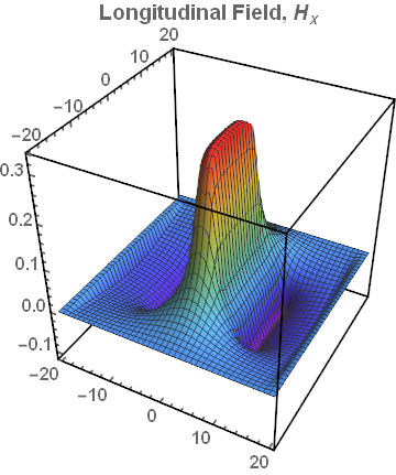
Lindholm's Equations use superposition to create a head model which simplifies the geometry to that of a finite track width, but semi-infinite poles. We will show example surface plots using the directional terminology chosen by Lindholm. The axes are labelled by grid points in the 'x' and 'z' direction.
The plot represents a single recorded transition in the media and, like all plots on this page, shows the gradient in the media as seen by the chosen head geometry.
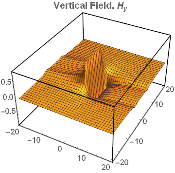
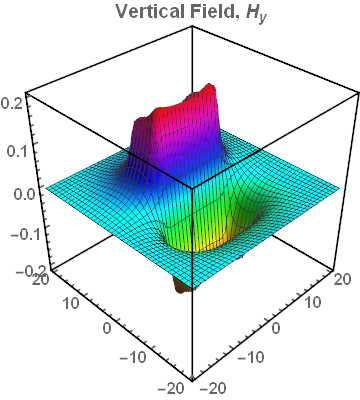
This plot shows the field at right angles to the media.
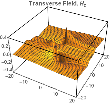
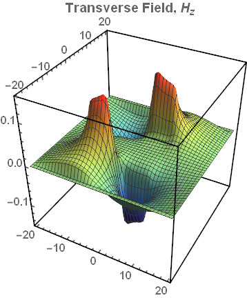
Here is a plot of the field across the track.
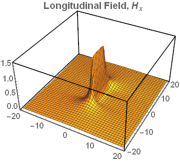
Unlike the Linfholm limitation of semi-infinite poles, these plots allow control over the pole length. Note the presence of undershoots on either side of the main pulse.